
Wrote by Wassim B., Cybersecurity Expert SQUAD
As illustrated in Figure 2, the proposed anomaly detector monitors VNFs (Section 1), preprocesses the monitored data (Section 2), trains models (Section 3), evaluates models’ performance and detects anomalies.
1) VNF Monitoring
VNFs are monitored by some agents that are deployed next to each VNF and collect the data status of each VNF. Examples of collected data include CPU load, network memory usage, packet loss, traffic load that are expressed in the form of time series.

Fig. 1 Proposed statistical ML-based anomaly detector
2) Data preprocessing
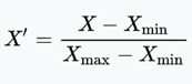
The raw data that are collected need to be processed, i.e., filtered and converted into an appropriate format. First, features are filtered, (i) removing those that do not distinguish abnormal states, (ii) eliminating redundant features that are intrinsically correlated with each other and therefore do not provide additional information. The filtered data (see Table 1) relate to the use of VNF resources and VNF services. Then, data are properly scaled using Min-Max feature normalization [20] that brings all features into [0,1] range. In particular, the normalized value x' is based on the original value x and the minimum and maximum values (xmin and xmax):
| Feature | Description |
| timestamp | Time of the event in the VNF resource usage |
| CurrentTime | Time of the event in the VNF service information |
| SuccessfulCall(P) | Number of successful calls at t time |
| container_cpu_usage_seconds_total | Cumulative CPU time consumed per CPU in sec |
| container_memory_working_set_bytes | Current working set in bytes |
| container_threads | Number of threads running inside the container |
3) Training and evaluating model’s performances
The proposed anomaly detector supports time series forecasting [16], which corresponds to the action of predicting the next values of a time series from its past values. As depicted in Figure 1, at any time t, an anomaly detector predicts what will happen in the near future [y’1,...,y’t] based on the past values [yt-1, …, yt-p] and [εt-1,..,εt-q].
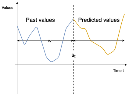
Our anomaly detector uses the statistical models, namely the AutoRegressive Integrated Moving Average (ARIMA), Seasonal AutoRegressive Integrated Moving Average (SARIMA) and Vector Autoregressive Moving Average (VARMA) [10][11]. Unlike existing approaches, we propose a parameterized window in order to predict both small and large durations. We also propose to run at the same time the different models with different size of the sliding window to cover different problems such as real time anomaly detection and anomaly detection verification. The advantage of this method is to have a small window for real time anomaly detection to keep only few data in the training set so as not slow down the execution of the model. But we also cover a large training data to check if we don’t miss anomalies in the real time part. The size of the sliding window w could not exceed the size training set st, i.e., st > w.
4) Detecting anomalies
Time series anomaly detection has largely focused on detecting anomalous points or sequences within a univariate or multivariate time series [39]. The problem of detecting anomalies can be formalized as follows: the aim is to detect a set of anomalies denoted by s ⊂Tst*f, where s is the set of anomalies, Ts is the multivariate time series, t is the length of the timestamp and f the list of features which compose the multivariate time series.
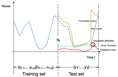
In order to detect anomalies we set up a fixed threshold calculated on all the predicted errors in the test set denoted by pe where pe = | v - y’t | , v is the real value and y’t is the forecasted value according to a model. The fixed threshold is calculated according to the three-sigma rule [35]. The so-called 3 sigma-rule is a simple and widely used heuristic for outlier detection [40]. To fix the threshold according to the three-sigma rule, we need to find the mean and the standard deviation of pe in the testing set, then multiplying the standard deviation by 3 and adding the mean.

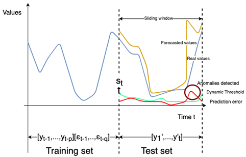
The dynamic threshold is calculated on the pe of the sliding window in the test set.
For the dynamic threshold, we will need two more parameters: a window which we will inside calculate the threshold and a coefficient that will be used instead of 3 from the three-sigma rule formula. For the dynamic threshold the parameters are empirically chosen. The dynamic threshold il calculated for each value of the window.

As depicted in Fig.3 and Fig. 4 a set of value v ⊂ Tst*f is detected as an anomaly when: . Finally, v is added to the set of detected anomalies as presented before denoted by s ⊂ Tst*f.
Evaluation:
As we are in a NFV environment, I set up a virtualized IP Multimedia Service from where we collected data status for 3 weeks. We need to evaluate the best model for each different situation as the data set presents seasonalities in the call distribution.
In order to evaluate the performance associated with our anomaly detector, we need to collect normal data and anomalous data, as anomalous data do not occur frequently on the network. I use anomaly injection techniques [19] to generate anomalies to test the anomaly detector. The anomaly injection was done by 1) injecting abnormal values where the VNF operates, and 2) simulating packet loss which does not guarantee the correct service operation. The first method causes anomalies directly in the Kubernetes [14] pods where the VNF operates. The anomalies are considered in terms of virtual resources such as CPU load/second usage and memory. The second method consists in causing anomalies directly in the VNF’s service. This may cause anomalies in the virtual service function and make the VNF not operate as intended.
Finally, in order to remain in a machine learning methodology, the dataset is divided into a training part to train the model and find the best combination of parameters and a test part to compare the predicted values with the original values.
Performance Indicators
The forecasted values for each time series generated by the models are assessed with three statistical performance measures, the Mean square error (MSE), the Root mean square error (RMSE) and the Mean absolute percentage error (MAPE) [36][37][38]. The best model is selected based on the lowest statistical value.
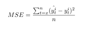
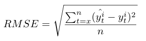
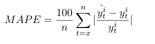
For the MSE, RMSE and MAPE, x is the first value of the training set or the sliding window and n is the last one. y^ti and y^ti are respectively the forecasted and the real value of the time series i.
Read the first two parts ⤵
References :
[1]Donovan, J., & Prabhu, K. (Eds.). (2017). Building the network of the future: Getting smarter, faster, and more flexible with a software centric approach. CRC Press.
[2]Nadeau, T. D., & Gray, K. (2013). SDN: Software Defined Networks: an authoritative review of network programmability technologies. " O'Reilly Media, Inc.".
[3]Hernandez-Valencia, E., Izzo, S., & Polonsky, B. (2015). How will NFV/SDN transform service provider opex?. IEEE Network, 29(3), 60-67.
[4] NFV White Paper, (2012), Network Functions Virtualisation–Introductory White
Paper., SDN and OpenFlow World Congress. October 22–24, 2012, Darmstadt, Germany.
[5]Cherrared, S., Imadali, S., Fabre, E., Gössler, G., & Yahia, I. G. B. (2019). A survey of fault management in network virtualization environments: Challenges and solutions. IEEE Transactions on Network and Service Management, 16(4), 1537-1551.
[6]Nouioua, M., Fournier-Viger, P., He, G., Nouioua, F., & Min, Z. A Survey of Machine Learning for Network Fault Management. Machine Learning and Data Mining for Emerging Trend in Cyber Dynamics: Theories and Applications, 1.
[7]Boutaba, R., Salahuddin, M.A., Limam, N. et al. A comprehensive survey on machine learning for networking: evolution, applications and research opportunities. J Internet Serv Appl 9, 16 (2018).
[10] Box, G. E., Jenkins, G. M., Reinsel, G. C., & Ljung, G. M. (2015). Time series analysis: forecasting and control. John Wiley & Sons.
[11]Brockwell, P. J., Brockwell, P. J., Davis, R. A., & Davis, R. A. (2016). Introduction to time series and forecasting. springer.
[12]Roh, Y., Heo, G., & Whang, S. E. (2019). A survey on data collection for machine learning: a big data-ai integration perspective. IEEE Transactions on Knowledge and Data Engineering.
[13]http://openimscore.sourceforge.net/
[14] What is Kubernetes ? - https://kubernetes.io/docs/concepts/overview/what-is-kubernetes/
[15]Turnbull, J. (2018). Monitoring with Prometheus. Turnbull Press.
[16]Hyndman, R. J., & Athanasopoulos, G. (2018). Forecasting: principles and practice. OTexts.
[17] Pena, D., Tiao, G. C., & Tsay, R. S. (2011). A course in time series analysis (Vol. 322). John Wiley & Sons.
[18] Reinsel, G. C. (2003). Elements of multivariate time series analysis. Springer Science & Business Media.
[19]Ziade, H., Ayoubi, R. A., & Velazco, R. (2004). A survey on fault injection techniques. Int. Arab J. Inf. Technol., 1(2), 171-186.
[20]Zheng, A., & Casari, A. (2018). Feature engineering for machine learning: principles and techniques for data scientists. " O'Reilly Media, Inc.".
[21]Lim, B., & Zohren, S. (2020). Time series forecasting with deep learning: A survey. arXiv preprint arXiv:2004.13408.
[22]Brownlee, J. (2018). Deep learning for time series forecasting: predict the future with MLPs, CNNs and LSTMs in Python. Machine Learning Mastery.
[23]Mathew, P. S., & Pillai, A. S. (2021). Boosting Traditional Healthcare-Analytics with Deep Learning AI: Techniques, Frameworks and Challenges. In Enabling AI Applications in Data Science (pp. 335-365). Springer, Cham.
[24]Reinsel, G. C. (2003). Elements of multivariate time series analysis. Springer Science & Business Media.
[25]Su, Y., Zhao, Y., Niu, C., Liu, R., Sun, W., & Pei, D. (2019, July). Robust anomaly detection for multivariate time series through stochastic recurrent neural network. In Proceedings of the 25th ACM SIGKDD International Conference on Knowledge Discovery & Data Mining (pp. 2828-2837).
[26]Nielsen, A. (2019). Practical time series analysis: prediction with statistics and machine learning. " O'Reilly Media, Inc.".
[27]Nason, G. P. (2006). Stationary and non-stationary time series. Statistics in volcanology, 60.
[28]Chatfield, C. (2003). The analysis of time series: an introduction. Chapman and Hall/CRC.
[29]Dickey, D. A., & Fuller, W. A. (1979). Distribution of the estimators for autoregressive time series with a unit root. Journal of the American statistical association, 74(366a), 427-431
[30]Phillips, Peter & Perron, Pierre. (1986). Testing for a Unit Root in Time Series Regression. Cowles Foundation, Yale University, Cowles Foundation Discussion Papers. 75. 10.1093/biomet/75.2.335.
[31]Watson, P. K., & Teelucksingh, S. S. (2002). A practical introduction to econometric methods: Classical and modern. University of West Indies Press.
[32]Akaike, H. (1998). Information theory and an extension of the maximum likelihood principle. In Selected papers of hirotugu akaike (pp. 199-213). Springer, New York, NY.
[33]Myung, I. J. (2003). Tutorial on maximum likelihood estimation. Journal of mathematical Psychology, 47(1), 90-100.
[34]Hartley, H. O., & Booker, A. (1965). Nonlinear least squares estimation. Annals of Mathematical Statistics, 36(2), 638-650.
[35]Pukelsheim, F. (1994). The three sigma rule. The American Statistician, 48(2), 88-91.
[36]Chai, T., & Draxler, R. R. (2014). Root mean square error (RMSE) or mean absolute error (MAE). Geoscientific Model Development Discussions, 7(1), 1525-1534.
[37]Allen, D. M. (1971). Mean square error of prediction as a criterion for selecting variables. Technometrics, 13(3), 469-475.
[38]De Myttenaere, A., Golden, B., Le Grand, B., & Rossi, F. (2016). Mean absolute percentage error for regression models. Neurocomputing, 192, 38-48.
[39]Blázquez-García, A., Conde, A., Mori, U., & Lozano, J. A. (2020). A review on outlier/anomaly detection in time series data. arXiv preprint arXiv:2002.04236.
[40]Lehmann, Rüdiger. (2013). 3sigma-Rule for Outlier Detection from the Viewpoint of Geodetic Adjustment. Journal of Surveying Engineering. 139. 157-165. 10.1061/(ASCE)SU.1943-5428.0000112.
[41]Diamanti, A., Vilchez, J. M. S., & Secci, S. (2020, September). LSTM-based radiography for anomaly detection in softwarized infrastructures. In International Teletraffic Congress.